DeltaV Predict

DeltaV Predict Algorithm

This section presents the technical background and implementation of Model Predictive Control (MPC) as implemented in DeltaV Predict. The applied predictive control algorithm has its roots in Dynamic Matrix Control (DMC) with significant modifications, such as prediction horizon-dependent penalty on error, control horizon-dependent penalties on moves, asymmetric funnel control, range control and reference trajectory. Controller robustness is substantially improved as a result of these enhancements.

Understanding the details of the MPC algorithm is not necessary to successfully use DeltaV Predict. Skip to the Using DeltaV Predict topic unless you have an interest in how the MPC algorithm and the associated process identification are implemented in DeltaV Predict.

Process identification is performed using two types of models: Finite Impulse Response (FIR) and Auto-Regressive (ARX). Model validation is accomplished by matching simulated and real process data. Constraints on the process outputs are handled by managing working setpoints of the controlled variables. Process optimization is achieved by maximizing or minimizing a selected process input until one manipulated variable approaches its limit. Such optimization is an inherent part of the MPC algorithm. The MPC algorithm is embedded in the DeltaV controller as a function block and is supported by DeltaV Predict.

Process Modeling and Identification

The process model is the basis of MPC technology. DeltaV Predict uses step response modeling for the MPC controller. This approach has been proven effective in numerous DMC applications. Step response modeling makes prediction of process outputs explicitly available for display in the application. The predicted error vector is computed as an input to the MPC controller. Displaying prediction to an operator is an important way to visually evaluate the process control. DeltaV Predict's operator interface displays the future process outputs. The MPC function block develops future process outputs as a process state and uses modified state space form for process modeling.

For a single input, single output (SISO) process, the future prediction of the process output can be calculated as follows:

x_k+1 = Ax_k + BΔu_k + FΔw_k

y₀ = Cx_k+1

where:

x_k = [y⁰, y¹, yⁱ,…y^{p -1}]^T is vector of future output prediction 0,1…, i,… , p-1 steps ahead at the time k

A is shift operator, which is defined as Ax_k = [y¹, y²,…yⁱ,…, y^p-1]^T

B = [b₀, b₁,…b_i,…, b_p-1]^T is vector of p step response coefficients

Δu_k = u_k - u_k-1 is change on the process input/controller output at the time instant k

Δw_k process output measurement - process model output, mismatch resulted from the noise, unmeasured disturbances, and model inaccuracy

F filter, p dimension vector with unity default values

C is the operator that takes the first component of the x_k+1 vector

For an n outputs and m inputs process, vector X_k has dimension n*p, and vector B is converted into a matrix with dimension n*p rows and m columns.

You can identify the step response model using two modeling techniques: FIR and ARX. Use the short horizon process model to identify the differential FIR model. For example, the following equation applies to the SISO process:

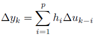
Where Δy_k = y_k - y_k-1 is the change on the process output at the time instant k.

p is prediction horizon, with a typical default value for MPC model 120. Identifying step response with full prediction horizon and as many as 120 coefficients causes overfitting and results in significant parameter uncertainty.

By using a short horizon with 30 or 40 points for the FIR model, you can avoid model overfitting. An FIR model with a short horizon provides an initial part of the step response and is adequate for defining dead times using a heuristic approach. The dead times are then used in a ARX model, which has significantly fewer coefficients than an FIR model. For example, the following equation applies to the SISO process:

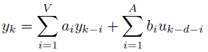
A and V are autoregressive and moving average orders of ARX with a default value of 4.

For a MIMO process, superposition is applied from each input (additive action) on every output both in FIR and ARX models.

Use an ARX model and apply unit step on one of the inputs to get step responses for that input. To get a complete model, repeat the procedure of applying unit steps for every input.

As a result of using this combined identification technique, an optimal process model is developed.

MPC Controller

The MPC controller minimizes the squared error of a controlled variable over prediction horizon and the squared error of controller output over control horizon:

min {||Γ^y[X(k) - R(k)]||² + ||Γ^uΔU(k)||²}

ΔU(k)

where:

The solution is in the form:

ΔU(k) = (S^uTΓ^yTΓ^yS^u + Γ^uTΓ^u)^-1S^uTΓ^yTΓ^yE_p(k)

where:

S^u = process dynamic matrix built from step responses, p × m for SISO model and p*no × m*ni matrix for MIMO model with ni inputs and no outputs

E_p(k) = error vector over prediction horizon

The performance of the control algorithm can be modified using the following adjustable parameters: p, m, Γ^u, and Γ^y. From an implementation standpoint, p and m are not convenient to use as tuning parameters. In DMC implementations, Γ^u and Γ^y are applied as scalars (that is, control error is multiplied by the scalar Γ^y over the whole prediction horizon), and any controller moves over control horizon are multiplied by the scalar Γ^u.

The robustness of the controller can be significantly improved by shaping Γ^y and Γ^u coefficients dependent on control error and control move predictions. Various functions can be used for shaping the coefficients of Γ^y - linear, exponential, and so on. The current implementation applies linear function with the option to set some initial coefficients to zero. The number of initial coefficients in Γ^y equal to zero is called the patience factor. The application of incremental penalty on error function is preferred when the initial part of a step response is uncertain but process steady gain is reasonably well defined.

Γ^u is a basic controller-tuning parameter defined at the controller generation phase. Increasing Γ^u makes control more damped, and, in reverse, decreasing Γ^u makes the control action more aggressive and control response faster. Another degree of tuning can be achieved by applying decreasing penalties on future moves. This makes the first controller move less aggressive since next moves are relaxed and can be used with less penalties for error correction. It is readily apparent that the second and next moves, in this case, can violate move constraints. This is not a practical concern since controller moves are recalculated during every scan and only the first move is implemented. As a result, the first move is smaller and controller robustness is increased.

In addition to shaping the controller structure at the generation phase, a number of features have been implemented to manage controller behavior and robustness online. Refer to the following figure.

One important tuning parameter is the setpoint filter, which is also known as the reference trajectory. The Predict trajectory acts in a different way than the trajectory currently used in other MPC products. Instead of penalizing any departure from the trajectory, only those deviations that are below trajectory or above setpoint value are penalized (Area A and Area C if control range = 0). In addition, the control error is considered zero if the control variable is within range (Area C with range > 0). These features constitute a funnel control, which can be shaped online by changing the setpoint filter time constant and range, which further enhances controller robustness and flexibiltiy.

During controller generation, all of the controller settings are calculated depending on process model, and there is no need for user involvement. However, if you identify yourself as an Expert using the Option selection in DeltaV Predict, you can change default controller settings to enhance specific features.

Output Constraints Handling

A typical MPC configuration includes both controlled and constrained variables. The MPC controller does not take action on constrained variables unless a predicted constraint variable violates the constraint limit. In that case, the MPC controller changes the working setpoint of the selected controlled variable on the value:

ΔSP_CV = -r*G_CV-AV*ΔAV

where:

ΔAV = the magnitude of the predicted steady state constraint violation

G_CV-AV = the gain relationship between constraint variable (AV) and CV

r = the relaxation factor, < 1

ΔSP_CV = the change in working setpoint of the controlled variable

The association between constrained variables and controlled variables is established during configuration. Therefore, the gain relationship is defined automatically from the process model. If the constraint limit violation ends, the working setpoint returns in a stepwise manner to the desired setpoint value.

Optimization

The objectives of optimization often include maximizing product value and minimizing raw material cost. In most cases where a linear model is applied for control, linear programming (LP) can be applied for optimization equally well. The Simplex algorithm or its modifications serves for the LP optimal solution. If a feasible solution exists, it is always located at one of the limit intersections. We use this result to perform simple optimization. This is done using a priori knowledge where we know there are optimization targets, such as the minimization or maximization of one of the production parameters within constraints on process inputs.

A typical MPC configuration can include three controlled parameters (CV), up to four constraint parameters (AVs), and up to four disturbances (DVs). To control three CVs, three manipulated variables (MVs) plus at least one additional MV are used for optimization. The extra MV controls a process input that sets up the optimized parameter for production rate or raw material cost. Finally, an extra CV is introduced, which is a shadow of the optimized MV. This is done by connecting the optimizing MV to an extra CV. In DeltaV Predict, we call this the optimizing CV. The MPC controller generated for this configuration becomes an optimizing controller. By setting the setpoint of the optimizing CV to a maximum (or minimum) achievable value of the optimizing MV, the MPC function block drives the optimizing MV toward optimal value at the setpoint of the optimizing CV until any of the manipulated variables (or, specifically, any predicted value of MV) violates an input limit. Then, the optimizing MV changes until all manipulated variables are within their input or output limits.