Using DeltaV Neural

Creating a Neural Network Module

Using DeltaV Neural to provide a continuous estimate of a process parameter begins with the creation of a DeltaV module that includes the Neural Network (NN) function block. Use the NN function block in conjunction with a Lab Entry (LE) function block where the parameter that is to be estimated by the NN block is currently only available through offline lab analysis. This offline lab analysis may be entered into your DeltaV system using the dynamo provided with the LE function block. Where the parameter of interest is periodically measured using an online sampled analyzer, use an Analog Input block to obtain the sampled value needed by the NN function block. In either case, the DeltaV Neural application uses the sampled measurement when training the neural network. Also, after the network is trained, the NN function block uses the sampled value to correct the continuous estimate of the current and future value of the parameter that is calculated based on upstream measurements.

After you decide on a process variable to model with a neural network, create a module in Control Studio. In the module, add an NN function block from the Advanced Control palette. If you are modeling a process that uses lab analysis data, add an LE function block. Through the configuration of the NN function block, you may specify the upstream measurements that you believe influence the estimated sampled parameter. You may specify as many as 20 inputs. You can assign a custom name to each input for display in the Neural application and the NN block dynamo. This name is used as the identifier for the input and must, therefore, be unique.

If the process variable to be estimated is currently measured using offline lab analysis, then include an LE function block wired to the NN function block. Otherwise, the analog input for the sample analyzer used for this measurement should be wired to the NN function block.

Commissioning a Neural Network Function Block

To commission a Neural Network function block complete the following tasks:

The Neural application appears as shown.

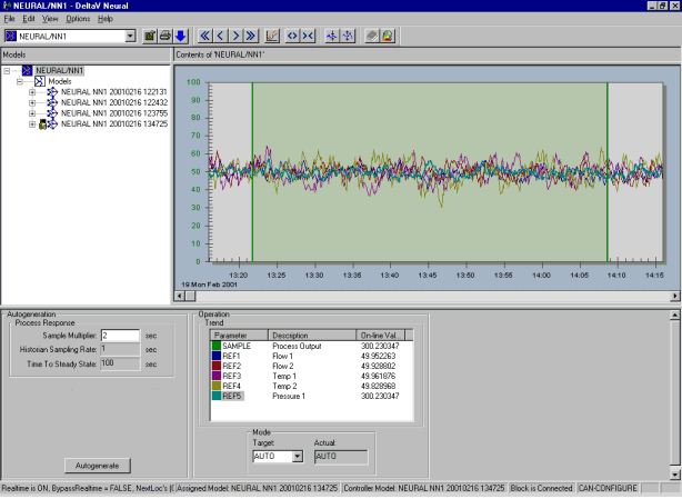
The referenced inputs (REF) parameters and the sampled (SAMPLE) parameter are trended automatically. Up to six of the neural network inputs can be trended at one time. For good data values, trends appear in the colors indicated in the parameter data area. The color varies to indicate questionable status (yellow for uncertain or limited values, red for bad values). To add or remove a parameter from the trend view, double-click the parameter in the Operation Trend pane. When you right-click a selected parameter, options are provided that allow you to modify the trend view (that is, change the trend range). You can use the toolbar controls or the slider bar to adjust the time window that is shown on the trend. Note that if the trend parameter list and trend view shows any inputs with an incorrect value of 0.0, it may be a result of configuring invalid reference inputs in the NN block.

Next, you need to enter a value for the Sample Multiplier to configure the Time to Steady State (TSS) - the estimated time (in seconds) for the process to completely respond to changes in inputs. This field also corresponds to the horizon over which DeltaV Neural estimates input delays.

The Time to Steady State (TSS) is calculated as:

TSS = 50 * Data Sampling Rate * Sample Multiplier.

The Data Sampling Rate (DSR) is the Historian Sampling rate entered in the NN function block Properties dialog. If you are using data from a file, the sampling rate in the file is read as the Data Sampling Rate for the TSS calculation.

The Sample Multiplier is the factor at which data from the given data set (created by sampling at the Data Sampling Rate) is sampled for creating the neural net model. For example, Sample Multiplier of one (1) means all the samples at the DSR are used, while Sample Multiplier of two (2) implies that only every second sample from the data set is going to be used for training - half of the former case. In effect, the product of DSR and Sample Multiplier establishes the effective sampling rate of the data to be used for training.

To modify the TSS, edit the Sample Multiplier according to the formula above. For example, if the Historian Sampling Rate is one second and the process TSS is estimated to be 100 seconds, set the Sample Multiplier to two (2). If you are using data from a file in which the sampling rate is two seconds, the minimum possible TSS is 100 seconds (Sample Multiplier = 1). Other possible TSS values are 200 seconds, 300 seconds, and so on for Sample Multipliers of 2, 3, and so on.

When using the NN block in conjunction with an LE block for lab analysis samples, note that the TSS value establishes the maximum sample delay that affects the NN block's automatic correction mechanism.

To form the data set to train the neural network, all input and output data should show reasonable variation (flat data lines have no effect) about the normal region of operation of the process. There should be sufficient data reflecting normal process operating conditions. If the time between samples is large, the data must be collected over a greater time. Generally speaking, the larger the data set, the better the resulting trained neural net. Also, NNs with a higher number of inputs require more data than smaller NNs. Once sufficient data is collected, select the historical data to generate the neural network. The green area on the trend view indicates the data used to generate the neural network. You can adjust the range by dragging the start and end bars or by right-clicking the trend to set the right or left edge of the green area. You can exclude other unwanted data within the selected data by right-clicking within the green and stretching the red band over the unwanted data. After you select the data, click Autogenerate to create a neural network for the process.

While the Neural application is generating the neural network, a line of status information appears in the Autogeneration area of the interface to show the progress.

When the minimum error is achieved, a pop-up message appears saying that the training is completed. The trained network is loaded into the NN function block in the database. The neural network model that is created is shown automatically in the left panel of the DeltaV Neural screen. A model overview of the calculated sensitivity is automatically displayed.

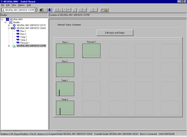
The sensitivities indicate how changes in the inputs affect the sampled measurement that is modeled by the neural network. Inputs that were determined to have insignificant influence on the sampled value are not used in the neural network and are indicated in the sensitivity display by a large red X shown in place of the sensitivity plot.

Double-click a sensitivity to see a more detailed view appear, as shown in the following figure.

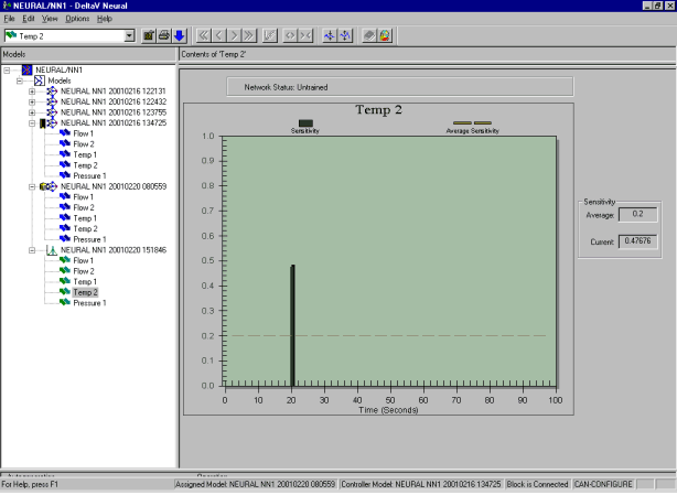
The vertical scale shows the sensitivity of the output to this input. (Note that the sum of the sensitivities for all inputs is 1.0.) The time scale shows the delay (the time it takes for a change in the input to be reflected in the output). The average sensitivity is shown as well.

Once you have viewed the input sensitivities and are satisfied that the important inputs were selected, download the associated module to utilize the trained network. If you would like input in the training of the neural network or more details on how well the neural network fits a set of process data, use the expert features of DeltaV Neural, as detailed in the following section.

Expert Option

You may provide greater input during the generation of the neural network by selecting the Expert option from the DeltaV Neural application. If you have selected this option, additional features are available in the application. The following figure shows the application window with the Expert option selected.

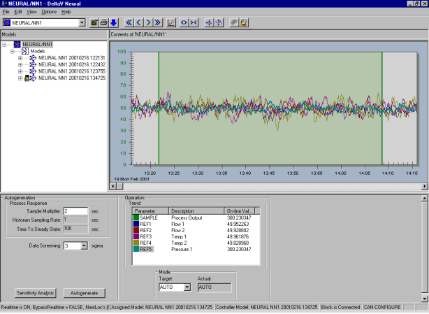
With the expert option selected, you can choose the data screening range by selecting a Data Screening value. This sets the limits on the data used for training based on the selected sigma (number of standard deviations) value. The default is 3.5 sigma, which means that the data training limit is Mean ±3.5 sigma, and values outside those limits are treated as outliers. These same limits are used during online operation of the neural net.

Also, with the Expert option selected, you can perform a Sensitivity Analysis (by clicking the Sensitivity Analysis button) to determine the sensitivity of the output to the inputs without training the neural network.

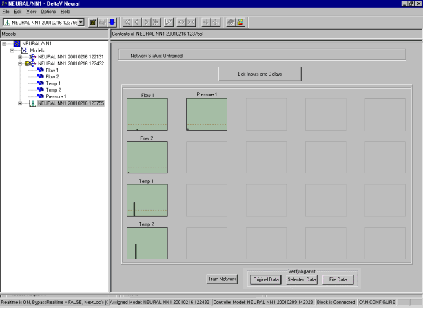
The sensitivity overview with the Expert option selected contains additional buttons you use to train and verify the network. Double-click a sensitivity to open a detailed view of that input sensitivity, as shown in the following figure.

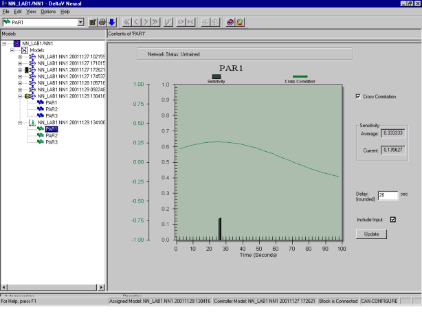
With the Expert option selected, the sensitivity detail contains more information and controls. The detail view shows the cross correlation between the input and the sampled output. The Neural application uses the peak value found for the cross correlation to determine the time delay associated with the input and its impact on the sampled value. If you are familiar with the process delay and time constants associated with the inputs, you may want to verify that your knowledge of the delay matches what was calculated. To try a different delay, enter the value in the Delay field, and then click Update. In response, the sensitivity is recomputed for the delay you entered.

If the sensitivity associated with an input is low, then you may want to remove it from use in the neural network. In many cases, such inputs have already been eliminated and are shown with a red X in place of the sensitivity. To eliminate an input from the generation of the neural network, click the Use Input check box to remove the check mark, and then click the Update button. If an input is shown as not selected but you would like to examine the calculated sensitivity, select the Use Input check box, and then click Update. In response, the sensitivity and cross correlation are displayed.

After you are satisfied with the inputs selected for use in the neural network, click the Train network button at the bottom of the sensitivity overview screen. You can also train a model by selecting it in the Hierarchy view, right-clicking, and then selecting Train Network from the pop-up menu. The Training Parameters dialog appears as shown in the following figure.

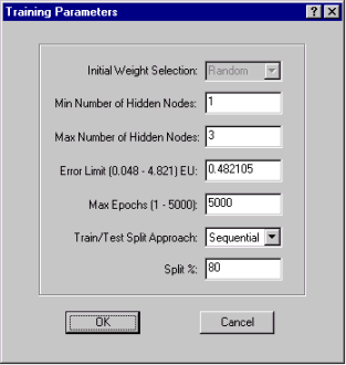
The dialog contains additional options you can use to modify the neural network training. If you have expert neural network knowledge, you can change the default values to address special requirements. For example, you can change the starting number of hidden nodes used in generating the neural network to determine the impact on the model accuracy. Click OK on the dialog after you are satisfied with the values.

Training begins, and another dialog appears that provides information about the training, as shown in the following figure.

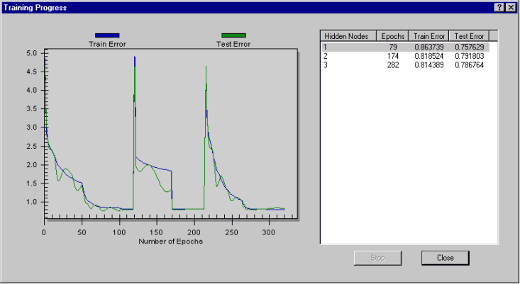
This dialog shows the neural network training progress and results. The graph shows the training error and test error values in Engineering Units as a function of the number of epochs. As hidden nodes are added, spikes appear as a result of random initialization of the network. The right pane of the dialog shows the network with the lowest error (test error) for each hidden node number. Among these, the best network is automatically selected by the Neural application as the trained neural network model. This is highlighted in gray at the end of training and is the network that is assigned to the NN block. Note that the random initialization of the network may result in different neural network configurations (as defined by the varying number of hidden nodes) being selected in the right pane for different training runs on the same data set.

After you train the neural network, you can verify how well the model fits the sampled data by clicking either selection in the Verify Against area at the bottom of the sensitivity overview. To verify against the data used to create the model, click Original Data. To verify against a different selection, open the Data view (select the block or Models in the Hierarchy view), select a data range, return to the sensitivity overview (click the model in the Hierarchy view), and then click Selected Data.

In response, a dialog appears that shows a plot of the actual values and predicted values calculated by the neural network, as shown in the following figure.

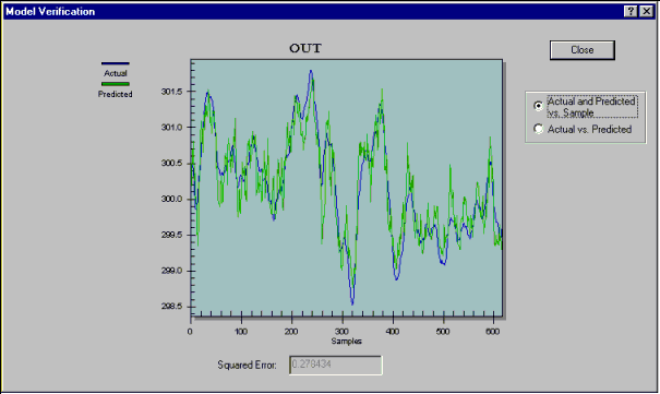
Use the squared error value shown at the bottom of the dialog in conjunction with the plotted data to determine how accurate the neural network model is for the selected data.

To see a plot of the actual vs. predicted values for the model, click the Actual vs. Predicted radio button. A plot of the calculated vs. sampled data appears as shown below.

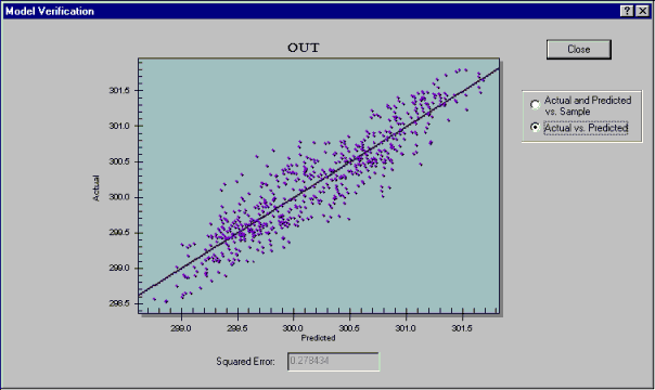
If the model is inaccurate, it may be the result of one or both of the following:

If autogeneration has eliminated an input which you know to have a significant influence on the parameter of interest, you can add that input to those used to train the neural network by selecting Use Input from the input detail sensitivity display.

To use the new neural network definition after training, you must download the associated module. All neural network function block parameters have assigned defaults. During online operation of the function block in Control Studio, you can adjust only those parameters of the block that do not impact the neural network model file. Also, you can change some parameters that are used during controller generation in offline mode. Any changes in these parameters require that the neural network be retrained in order for the changes to be used in the neural network model.

Defining a Neural Network Operator Interface

You can create an operator interface for the NN function block using predefined dynamos. You can access these dynamos under the NN set in the DeltaV Dynamo Reference Library.